Audio Forensics

Eight instruments for reading audio provenance — waveform dynamics, spectrogram, spectral profile, noise floor, MFCC trajectory, dynamics, spectral flux, and feature summary. A teaching tool for understanding how statistical audio analysis works.

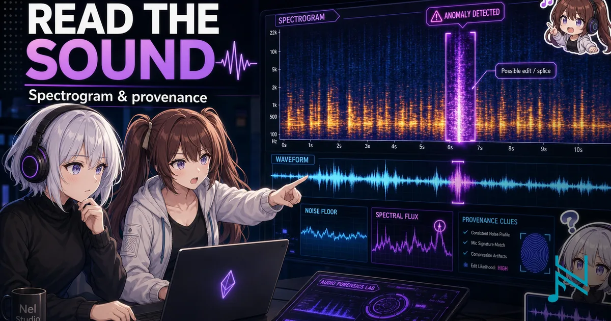
Every audio signal carries a statistical fingerprint. Not in what you hear, but in the numbers underneath.

The shape of the spectrum, the smoothness of the MFCC trajectory, the variance of spectral flux between frames. These patterns differ between a recording of physical acoustics, a digital synthesiser render, and a diffusion model's vocoder output.

Audio forensics is the science of reading those patterns.

These instruments are naive implementations using standard signal processing features: Meyda's MFCC, manual STFT, per-frame spectral statistics.

They demonstrate the logic of audio forensics and give you something concrete to interact with. A production classifier would train on thousands of labelled audio pairs, use learned embeddings rather than hand-computed features, and validate against adversarial examples.

What you see here is the approach, not the capability.

All analysis runs in your browser. No audio data is uploaded or transmitted. Decoding and feature extraction happen locally via the Web Audio API and Meyda.

Audio Forensics Tool

Audio A

116 D-min

Bury the Light

Bury the Light (vocals)

No audio loaded

Audio B

116 D-min

Bury the Light

Bury the Light (vocals)

No audio loaded

How a computer hears audio

To a computer, audio is a sequence of numbers -- a Float32Array of pressure values sampled at a fixed rate (44,100 times per second for CD quality).

There is no concept of "this sounds like a guitar" or "this sounds AI-generated." There are only those numbers.

Everything on this page is a mathematical operation on that sequence. The question is not "does this sound real?" but "do these numbers behave like a diffusion model's output, or like a synthesiser's?"

How AI audio is generated

Most current AI music systems (Suno, Udio, MusicGen, AudioLDM) learn patterns on mel spectrograms, IE: compressed visual representations of sound, rather than on raw waveforms.

Generating a track means generating one of those images (yes, AI creates the image of the sound you gonna hear later), then converting it back to audio using a vocoder.

That conversion step is where the forensically detectable artifacts appear.

Step	What happens	Analogy	What gets lost	Forensic consequence
Record / synthesise	Real acoustic event or DAW plugin produces a waveform with precise phase relationships between harmonics	The original painting — every brushstroke is there	—	Phase encodes the physics of the source
Mel spectrogram	Waveform is compressed into a 2D image: time × mel frequency bins. Amplitude is preserved; phase is mostly discarded	A photograph of the painting — composition intact, brushstroke texture gone	Phase information	The representation is lossy — reconstruction must invent what was discarded
Diffusion model	Model learns to generate plausible mel spectrograms from text prompts, trained to produce smooth gradual changes	An artist who has only ever seen photographs, now asked to paint from scratch	Sharp note-boundary transitions	MFCC trajectories are unnaturally smooth; spectral flux variance is lower than real synthesis
Vocoder decode	Learned algorithm reconstructs a waveform from the mel spectrogram, inventing phase	Recreating the canvas from the photograph — colours match, brushstrokes are guessed	Cannot recover physical phase relationships	Characteristic smearing above 4–8 kHz, visible in spectrogram; shimmer in broadband noise
Loudness normalisation	Platform applies gain to hit −14 LUFS target before delivery	Printing every photo at the same exposure regardless of the original lighting	Dynamic range	Compressed crest factor; waveform looks uniformly dense

What each instrument reads

Instrument	What the computer measures	DAW render	AI (diffusion vocoder)
Waveform	Peak-envelope amplitude over time; crest factor (peak ÷ RMS)	High crest factor if unmastered; natural amplitude variation	Lower crest factor — loudness-normalised before delivery
Spectrogram	Power at each frequency over time (STFT)	Clean harmonic series from synthesised instruments; discrete note attacks	Horizontal smearing above 4–8 kHz from vocoder phase reconstruction; blurred harmonic lines
Spectral Profile	Average power spectrum across all frames; centroid, rolloff, flatness	Determined by synthesis engine and mixing decisions	Characteristic rolloff shape from mel filterbank + vocoder bandwidth limit
Noise Floor	10th-percentile power at each frequency bin	Near-zero digital floor (no sensor noise in DAW renders)	Near-zero digital floor — same as DAW; this tab distinguishes both from mic recordings
MFCC	13 Mel-Frequency Cepstral Coefficients over time	Stochastic variation at note boundaries; sharp transitions from synthesiser envelopes	Unnaturally smooth trajectories — diffusion model learned gradual spectral evolution
Dynamics	Per-frame RMS energy; dynamic range; loudness histogram	Wide dynamic range if unmastered; natural energy contour	Compressed dynamic range (6–10 dB typical); uniform loudness histogram
Spectral Flux	Frame-to-frame change in magnitude spectrum; onset detection	Sharp onsets at note attacks; high flux variance	Smoother flux; fewer high-magnitude onset peaks
Feature Profile	All of the above as summary statistics	—	—

The samples

The preset samples are two recordings of the same composition:

DAW sample — a direct render from a digital audio workstation. No physical microphone. Clean digital floor. Unmastered. The dynamic range and spectral balance reflect the raw mix, not a commercially delivered track.
AI cover — a Suno generation referencing the same composition, produced using prompts from the Suno Builder tool on this site. Delivered at streaming loudness. Generated via diffusion model with vocoder decode.

What this comparison can and cannot show:

Tab	Diagnostic for AI vs DAW?	Confound
Waveform / Dynamics	Partially	Detects mastering decisions as much as generation method — unmastered DAW will have wider dynamic range than normalised AI regardless of origin
Spectrogram / MFCC	Yes	Vocoder artifacts and MFCC smoothness are independent of mastering
Spectral Flux	Yes	Onset sharpness reflects generation method, not post-processing
Noise Floor	No (for these samples)	Both are digital sources — neither has sensor noise; the tab is meaningful when comparing either to a microphone recording
Spectral Profile	Partially	Rolloff shape is partly a vocoder fingerprint, partly a mix/EQ decision

Tools of the trade

Understanding the analysis is easier once you know what tools were used at each stage of production, and what traces they leave.

Mixing

Tool	What it does	Forensic signature
EQ (equaliser)	Boosts or cuts specific frequency bands; shapes tonal balance	Spectral profile shows shelves and notches at the cut/boost frequencies; centroid shifts
Compression	Reduces dynamic range by attenuating peaks above a threshold	Lower crest factor; waveform looks more uniform; dynamics histogram narrows
Reverb / delay	Adds spatial impression by convolving with a room impulse response or feedback	Spectrogram shows frequency-dependent decay tails after transients
Saturation / distortion	Adds harmonic content by soft-clipping the signal	Spectral profile shows energy added at harmonics; flatness increases
Panning / stereo width	Places audio in the stereo field	Affects inter-channel amplitude ratio; not visible in mono-channel analysis on this page

Mastering

Tool	What it does	Forensic signature
Multiband compression	Independent compression per frequency band; often used to tighten low-end	Spectral profile becomes more uniform across bands; per-band dynamic range narrows
Limiter	Hard ceiling on peak amplitude (used to maximise loudness)	Very low crest factor; waveform flat-topped near 0 dBFS; peak and mean RMS converge
Loudness normalisation (LUFS)	Adjusts overall gain to a target integrated loudness (e.g. −14 LUFS for streaming)	Predictable RMS level; dynamic range preserved but absolute level is standardised
Stereo enhancement	Widens stereo image via mid/side processing or Haas effect	Not visible in single-channel analysis
Dithering	Adds shaped noise to mask quantisation artifacts when reducing bit depth	Adds a characteristic noise floor shape in the high frequencies

What AI generation replaces

Stage	Human workflow	AI (Suno / diffusion model)
Composition	DAW arrangement, MIDI, synthesis	Prompted from text; no MIDI or per-instrument tracks
Mixing	Manual EQ, compression, panning per track	Implicit — baked into the model's training distribution
Mastering	Separate mastering chain, LUFS targeting	Loudness normalisation applied at delivery; no separate mastering stage
Codec / delivery	Export to MP3/WAV/FLAC	Vocoder decode → MP3 at platform bitrate

The key forensic consequence: an AI audio has no explicit mix or master.

A spectral characteristic was learned jointly, not applied as a discrete step. This is why the vocoder artifacts appear simultaneously with the loudness normalisation signature.

What should I look for?

Principle	Applied to audio forensics
Converge across instruments	No single feature is conclusive. Spectrogram smearing + smooth MFCC + compressed dynamics all pointing the same direction is a composite case. One anomaly can't tell you if something is AI.
Control for mastering	Dynamics and waveform tabs reflect mastering as much as generation method. Compare only tracks at similar loudness targets, or treat dynamics as a secondary signal.
The baseline is the source	Diffusion model fingerprints differ by architecture: Suno, Udio, MusicGen each have characteristic spectral shapes. A classifier trained on one architecture won't generalise to another without retraining.
Digital is not AI	DAW renders, digital synthesisers, and sample-based music all have near-zero noise floors and clean digital characteristics. These instruments cannot distinguish digital synthesis from AI generation based on the noise floor alone.
Adversarial training is closing the gap	Vocoders trained with perceptual losses are reducing spectral smearing artifacts. The most durable tells are MFCC smoothness and spectral flux variance. They require learning genuinely different generation dynamics to fake, not just perceptual filtering. But with good enough learning, even current forensic tools eventually fail.

What a real audio forensics pipeline looks like

Component	What this page uses	What production uses
Feature extraction	Meyda per-frame features (MFCC, spectral flux, RMS) — hand-selected, 13 coefficients	Learned embeddings from models like CLAP, EnCodec, or AudioMAE — trained on millions of audio examples, capturing patterns no human specified
Classifier	None. We cannot load a giant classifier model in your browser and we dont want to use our cloud resources.	Trained binary or multi-class classifier with calibrated probability estimates; validated on held-out test sets from multiple model families
Temporal modelling	Per-frame statistics averaged or plotted — no sequence model	LSTM, Transformer, or conformer over the full feature sequence — detects patterns that span multiple seconds, not just single-frame statistics
Vocoder fingerprinting	Not implemented	Each vocoder architecture (HiFi-GAN, EnVoice, DAC) has a characteristic phase-reconstruction pattern detectable by a model trained on its outputs
Adversarial robustness	Not tested	Red-teamed against: pitch shifting, time stretching, re-encoding at different bitrates, adding noise, re-recording through a speaker

Glossary

Term	What it means
Waveform	The raw audio signal — a sequence of pressure values over time. What you see when you open an audio file in a DAW. Amplitude on the Y axis, time on the X axis.
Sample rate	How many times per second the pressure is measured. 44,100 Hz (44.1 kHz) is CD quality — 44,100 numbers per second per channel. Why? Because it is the Nyquist frequency of the human hearing, that is 20kHz.
dBFS	Decibels relative to Full Scale. 0 dBFS = the loudest possible digital value. Everything else is negative. −6 dBFS is roughly half the peak amplitude.
RMS	Root Mean Square — the square root of the average of squared amplitude values. A proxy for perceived loudness, more meaningful than peak.
Crest factor	Peak amplitude ÷ RMS, expressed in dB. High crest factor = lots of headroom between quiet and loud moments (natural). Low = compressed or limited.
LUFS	Loudness Units relative to Full Scale. A perceptually weighted loudness measure. Streaming platforms (Spotify, YouTube) normalise to −14 LUFS.
Fourier transform / STFT	A mathematical operation that decomposes a signal into its frequency components — "how much of each frequency is present." STFT (Short-Time Fourier Transform) does this in short overlapping windows to track how the frequency content changes over time.
Spectrogram	A 2D visualisation of the STFT result: time on the X axis, frequency on the Y axis, energy (loudness at that frequency) shown as colour or brightness. A sustained note shows as a horizontal band; a transient (drum hit) shows as a vertical streak.
Mel scale	A perceptual frequency scale. Human hearing distinguishes pitches more finely at low frequencies than at high frequencies. The mel scale compresses the high-frequency range to reflect this — 1 kHz vs 2 kHz sounds like a bigger jump than 8 kHz vs 9 kHz, even though the Hz difference is the same.
Mel spectrogram	A spectrogram whose frequency axis is on the mel scale, and frequency bins are grouped through triangular mel filterbanks. Used by AI systems because it matches how humans perceive pitch. The compression discards fine phase detail.
Vocoder	Originally a device for encoding and reconstructing speech. In modern AI audio: a neural network that converts a mel spectrogram back into a raw waveform. HiFi-GAN and EnCodec are widely used examples. The vocoder must invent phase that the mel spectrogram discarded.
Phase	The timing offset of a wave cycle relative to a reference. Two sine waves at the same frequency but different phases sound identical in isolation but interact (add or cancel) when mixed. Real acoustic instruments produce harmonic phase relationships determined by physics; vocoders invent them.
MFCC	Mel-Frequency Cepstral Coefficients. A compact description of the shape of the spectrum at a given moment — roughly, the "texture" of the sound. Computed by: mel spectrogram → log → inverse Fourier transform → first 13 coefficients. Widely used in speech recognition and audio classification. Coefficient 0 tracks loudness; coefficients 1–12 track timbral shape from broad to fine.
Spectral centroid	The frequency-weighted average of the power spectrum — the "centre of mass." Low centroid = bass-heavy / dark sound. High centroid = treble-heavy / bright sound.
Spectral flatness	Ratio of the geometric mean to the arithmetic mean of the power spectrum. Near 0 = tonal (energy concentrated at discrete harmonics). Near 1 = noise-like (energy spread evenly across frequencies).
Spectral flux	The frame-to-frame change in the magnitude spectrum. High flux = rapid spectral change (note attacks, transients). Low flux = sustained, static content. Used here to measure onset sharpness.
Noise floor	The residual energy present in a signal even during silence. For microphone recordings, this is dominated by preamp and sensor noise. For digital sources (DAW renders, AI audio), it reflects codec quantisation noise — much lower and shaped differently.
Diffusion model	A generative model trained to iteratively remove noise from a noisy input. At inference, it starts from random noise and progressively refines it into a structured output (image, mel spectrogram, etc.). Suno, Udio, and MusicGen use variants of this approach.
Modulation spectrum	The spectrum of the amplitude envelope of a frequency band — "how fast is the loudness of this frequency band oscillating?" A peak in the modulation spectrum at 50–200 Hz in the high-frequency band indicates periodic amplitude ripple: the vocoder shimmer artifact.